In the world of nutrition, mathematical models serve as powerful tools to study animal dietary requirements. These models play a pivotal role in helping us understand and predict precisely what animals need for optimal growth and development. In this post, we’ll explore a noteworthy mathematical model tailored for estimating amino acid requirements in pregnant sows—namely, the NRC (2012) gestating sow model. What makes this model particularly intriguing is a unique component: the enigmatic “time-dependent protein deposition.” This mysterious entity represents protein deposited by pregnant sows, yet its destination and functions remain unknown. Let’s investigate what the ‘time-dependent protein deposition’ is and how this may be an artifact of data interpretation.

The NRC (2012) gestating sow model

The National Research Council (NRC) which is the operating arm of the United States National Academies of Science, published a model in 2012 to determine optimal dietary protein and amino acid requirements for pregnant sows [1]. This model involves a series of calculations summarized as follows:

1. It calculates the amount of protein retained by the animals during gestation. This estimation includes protein retention in various tissues such as lean tissue, placenta, uterus, mammary gland, and the growing fetus for each day of gestation.
2. The model incorporates a factor to account for protein excretion, typically around 50%. This factor is then applied to calculate the overall protein requirement. For instance, if, on day 50 of gestation, the sow retains 70 g of protein, the model suggests providing 140 g in total. This is because 70 g will be retained, while the other 70 g will be excreted. The model conducts similar calculations for each essential amino acid.

Nevertheless, when calculating the protein retained in the different tissues (step 1 above), there was one protein pool that had no explanation, which was termed as the time-dependent protein deposition (figure 1).

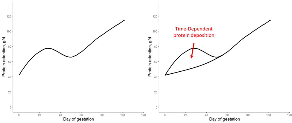
Figure 1. A. Simplified version of the protein deposition calculated by the NRC (2012) gestating sow model [1]. B. The protein retention is expected to increase across gestation, but there is some unexplained protein deposition pool termed as the time-dependent protein deposition.

What is the Time-dependent protein deposition?

The protein retention model in pregnant sows described above was developed based on a literature review performed by the NRC (2012) [1]. Nevertheless, there was no data available for the first 30 days of gestation, and assumptions had to be made. The NRC (2012) assumed reduced protein retention during the first days of gestation. As shown in the animation below, it seems that this assumption of reduced protein deposition during the first days of gestation caused the emergence of time-dependent protein deposition. When the assumption of reduced protein deposition at breeding is not considered, the relationship between the day of gestation and protein retention becomes quadratic.

A similar assumption regarding amino acid requirements was made by both American and French researchers. The model used for estimating AA requirements in the NRC (2012) and the INRAE (French National Research Institute for Agriculture, Food, and Environment) differs only by 3% [2]. However, the amino acid requirements calculated by Brazilian researchers take a different approach. They do not rely on the assumption of reduced protein deposition during early gestation and, as a result, recommend increased AA intake levels during this period [3]. Which set of predictions is more accurate: the ones made by the Americans and the French or the Brazilians? This is a topic we will explore in a future post.

“The Strange Case of Time-Dependent Protein Deposition” is an illustrative example highlighting that scientific models, both mathematical and conceptual, are often built on assumptions due to limited or incomplete information. It underscores the importance of recognizing the extent to which scientific knowledge relies on these assumptions, ensuring that we remain cognizant of the possibility that some scientific claims may not be absolute “facts.” The realm of biology, in particular, is replete with analogous situations where certain scenarios remain unverified through empirical evidence. However, these scenarios are sometimes treated as established facts due to a lack of comprehension regarding the underlying mental, conceptual, and mathematical models.

It is crucial to acknowledge that we build upon the foundation laid by eminent scientists who developed these models, including the NRC (2012), INRAE models, and the Brazilian tables for Poultry and Swine. These researchers have made invaluable contributions to the field of science. Consequently, we bear the responsibility of advancing science further while respecting their pioneering efforts. However, one recommendation for future models is to explicitly articulate the underlying assumptions that form the bedrock of these models. This transparency will facilitate the work of future scientists as more data becomes available. Moreover, it will enable users to discern the conditions under which the model predictions may hold true and when they may not. This approach fosters a more informed and robust scientific community.

Thanks for reading, and I hope you found this post helpful!

Christian Ramirez-Camba
Ph.D. Animal Science; M.S. Data Science

1.           NRC, Nutrient Requirements of Swine: Eleventh Revised Edition. 2012, Washington, DC: The National Academies Press. 420.

2.           van Milgen, J., et al., InraPorc: a model and decision support tool for the nutrition of growing pigs. Animal Feed Science and Technology, 2008. 143(1-4): p. 387-405.

3.           Ferreira, S., et al., Plane of nutrition during gestation affects reproductive performance and retention rate of hyperprolific sows under commercial conditions. Animal, 2021. 15(3): p. 100153.

Big data has been touted as a solution for addressing numerous challenges across various domains, including the field of livestock production. Through the analysis of extensive big data sets containing historical production data, the goal is to unveil concealed patterns. This, in turn, could lay the groundwork for improvements in our production systems. However, a poor understanding of this tool can lead to precisely the opposite outcome. Because the results and analysis are based on a large number of animals, it may give us the illusion that our results must be accurate, hiding system inefficiencies, directing our efforts away from the main problems.

What is Big Data?

The definition of big data can vary depending on the context. To simplify the concept, we can consider big data as a database that programs like Microsoft Excel cannot process, either due to the sheer volume of data it contains or the speed at which this data needs to be queried. In such cases, Microsoft Excel would struggle to handle it, making our work more challenging. For the purposes of this post, I’ll further simplify the concept of big data as a dataset related to pig production that includes information on tens of thousands of animals.

Size Doesn’t Matter; It’s How Well You Can Use It

When it comes to data analysis, the quality of the data being analyzed is more important than the quantity. Having, for example, 40,000 animals in a study doesn’t automatically enhance the quality of the conclusions. In fact, a large number of animals can actually have a negative impact on data interpretation, particularly in systems with standardized practices, as it can create a false sense of certainty.

To illustrate this point, let’s consider an example from the banking industry. When financial institutions create models to assess the likelihood of various customer groups repaying loans on time, they intentionally lend to customers they know won’t be able to repay. Additionally, these institutions grant loans that are much higher or much lower than what their system recommends lending. This approach allows banks to study how the population’s responses vary. These observations are then used to obtain insights into the behavior of the system, thereby facilitating the development of predictive analytics models. These models, in turn, assist in making forecasts for similar customer groups in the future.

Now, returning to the field of animal production, particularly in swine production, historical data is typically rooted in highly standardized practices that leave little room for variation. The three main inputs in swine production—feed, genetics, and facilities—tend to operate within very narrow margins. Diets are often quite similar due to the nutrient requirements concept, and data on the responses of different genetic lines are often limited. Also, facilities are pretty much the same, focused on providing the same conditions. These three variables account for between 85% to 95% of the inputs of the system, which are basically static.

Therefore, if our historical data (big data) is based on identical animals following identical standardized practices, and our goal is to investigate the cause of a specific effect (such as piglet mortality), our conclusion is likely to be predominantly influenced by the variable with the most variability. In swine production, management is one of the variables that exhibits a high degree of fluctuation. Many studies have concluded that management is primarily responsible for issues such as pig mortality faced by the swine industry. However, when factors like management and other variables with a relatively minor impact are rigorously controlled, their impact on pig mortality is accordingly small.

It’s essential to recognize that other underlying causes may remain concealed due to a lack of observable responses. These latent responses cannot surface because we are not allowing the system to reveal them. This is analogous to accepting null hypotheses without the presence of associated p-values—it involves concluding an effect does not exist simply because we haven’t observed it. Nevertheless, our methods are not allowing the patterns to emerge. Conducting research within commercial facilities presents significant challenges, particularly because accountants often resist altering the established production flow with the mindset of “If it ain’t broke, don’t fix it.” However, can we consider a pig production system with over 30% pig removals as not already broken?

Data regarding the microbiome can also be considered as big data. In this case, instead of having production data from thousands of animals, we have thousands of chunks of data (e.g., bacteria) from a few animals. Although I will dedicate a different post to this topic, we are expecting that the microbiome will have the answers we are looking for. After all, the microbiome does fluctuate in our static system. We hope that one day it will give us the answers we are looking for, especially since it is becoming increasingly cost-effective.

This scenario reminds me of the streetlight effect, which is a type of observational bias that occurs when people only search for something where it is easiest to look, and it is linked to a well-known joke:

“A policeman sees a drunk man searching for something under a streetlight and asks what the drunk has lost. He says he lost his keys and they both look under the streetlight together. After a few minutes, the policeman asks if he is sure he lost them here, and the drunk replies, no, and that he lost them in the park. The policeman asks why he is searching here, and the drunk replies, ‘this is where the light is.'”

We may be looking for the keys by the streetlight. Don’t get me wrong, changes in the microbiome do lead to improvements in pig survival and other variables. However, most, if not all, interventions have positive effects, although they are relatively small compared to the scale of the problem. This is mainly because pigs are so undernourished that almost any intervention appears to yield positive results (which is also a topic for a future post, but for further reference, please see this previous post).

Statistical Power

In data analysis, what the data doesn’t reveal is just as crucial as what it does. It’s essential to examine our assumptions to understand what aspects of the system we might be neglecting. We must recognize that we cannot simply accept null hypotheses or conclude that a variable has no effect when we lack the appropriate number of observations (sample size) or when the system doesn’t exhibit a significant range of variation (effect size) for investigation. In essence, for any type of data analysis, including big data, we need to conduct power test calculations, which encompass considerations of sample size and effect size, before investing our time in analyzing data and drawing potentially misleading conclusions from low-quality data. Defining the effect size can be challenging, and it should be a primary concern for biologists when analyzing big data. The determination of effect size for a power test depends on expertise within the specific field of knowledge.

In summary, having thousands of observations doesn’t automatically enhance the validity of conclusions. To evaluate the quality of these conclusions, we must assess the quality of the data by examining which variables in the system were allowed to fluctuate and to what extent. This context is crucial for drawing meaningful conclusions. In production systems, certain variables do naturally fluctuate, and we often attribute the responses under study to these variables, such as the microbiome or management practices. However, we may not truly understand how to predict or modify these factors to influence the system’s behavior. These variables do not appear to be the primary cause of the problem; instead, they often show minor, weak correlations with limited impact on the system. It’s vital to comprehend the nature of the problem at hand so that we don’t end up searching for the keys at the streetlight.

Thanks for reading, and I hope you found this post helpful!

Christian Ramirez-Camba
Ph.D. Animal Science; M.S. Data Science

In animal agriculture, a common practice involves conducting studies in research facilities and subsequently extrapolating their findings to broader populations. These studies are typically carried out by either an organization’s Research and Development Department or by external companies, which then use the study results to inform their strategies or product decisions. However, it’s worth noting that in numerous instances, these research teams exhibit deficiencies in their comprehension of the statistical methods they employ and a limited grasp of the dynamics within the various layers of the swine industry (i.e., pig> research barns> production barns).

As discussed in a previous post, a good example concerns the recommendation of using low-protein diets. In a traditional experiment aimed at assessing the effect of reducing dietary crude protein while supplementing with crystalline amino acids or other ingredients, the common conclusion is that “reduced protein diets cause a decrease in nitrogen excretion with no effect on animal performance.” However, it’s essential to recognize that this conclusion is opinion-based rather than scientific. In these experiments, it is typical to reduce dietary crude protein by 2 to 3% and supplement it with additives. However, to detect whether this reduction in dietary crude protein has a significant impact on pig growth or mortality, statistical power calculations indicate that more than 100,000 animals per group may be needed. Consequently, these types of experiments often lack the resolution or resources necessary to detect the effects of their interventions, leading to the erroneous conclusion that the intervention has no effect. Some companies and research groups go even further, advising producers to reduce protein, feed intake, energy, or other nutrients by 0.5 to 3% without adding any additives to achieve optimal “economic output”. In these scenarios, other effects are often completely disregarded. As explained further below, reducing nutrient intake does indeed influence pig survival, but this is frequently overlooked due to a limited understanding of statistical methods and animal biology, resulting in economic losses and welfare concerns.

The examples mentioned above can be misleading for producers and nutritionists due to a common misunderstanding of p-values. In experimental research, the absence of statistical significance (P > 0.05) does not necessarily indicate the absence of real effects. From a practical perspective, p-values have limitations and often reflect an evaluation of the methods used rather than a true biological response. When a study fails to detect statistical differences, it typically signifies that the methods employed may not have been suitable for detecting those differences. This could be due to a small sample size, inappropriate statistical techniques, or, more commonly, a combination of both factors.

It is possible to conclude that an intervention has no effects on pig “performance” if a power test is conducted before the experiment. However, another prevalent issue in these studies is the poor definition of “performance.” Often, power tests are exclusively performed on growth-related variables, while other crucial factors such as mortality, longevity, and health-related variables are overlooked.

To accurately conclude that an experiment did not affect “performance,” power tests must encompass ALL variables linked to pig performance, rather than focusing solely on growth-related parameters or the variable that the researcher deems “important.” As elaborated upon below, this skewed approach has led to an increase in pig removal rates. These experiments, concentrating solely on growth, neglected other critical responses, obtained p-values supporting their hypotheses, and erroneously applied the data from research barns to production sites. What appears to be transpiring is that certain effects, not initially evident in small sample studies, manifest their consequences in larger populations, contributing to the elevated pig mortality rates observed across the swine industry.

Thus, we inadvertently increase pig mortality due to a poor understanding of statistical methods, leading us to overlook certain effects because the studies lacked the capacity or resolution to detect them in the first place. Consequently, we end up extrapolating flawed ‘science’ to larger populations, causing considerable harm. Additionally, when a non-significant p-value (P > 0.05) conceals the mortality effect, survivor bias becomes more pronounced. In other words, if our interventions unintentionally kill the weakest animals, our practices may appear effective when we analyze data from the survivors, who are typically the heavier and more robust animals. Consequently, if we ‘correct’ the data by ignoring mortality, we mistakenly perceive ourselves as an industry that produces [surviving] pigs very efficiently. However, this false sense of efficiency is fundamentally rooted in a poor understanding of the system.

A Short Comment On Statistical Models

In the previous examples of experiments, the commonly employed methodology often utilizes ANOVA. However, this method is often inappropriate because animal responses, such as growth, survival, and health, are continuous variables (numeric), just like nutrient supply factors such as dietary protein, amino acids, and energy. In such cases, ANOVA becomes inadequate for reasons explained in a previous post, rendering the conclusions drawn from this method invalid.

Furthermore, complex systems like pig populations often exhibit non-linear dynamics. Consequently, linear models (e.g., linear and quadratic) are frequently unsuitable for studying these intricate dynamics. It is imperative to employ non-linear models to understand these systems better. However, it’s worth noting that non-linear models often yield p-values that are not meaningful in many cases.

If we are committed to a deeper understanding of these systems, we must move beyond a reliance on p-values. Alternatively, if p-values are to be used, they should be interpreted with a profound understanding of their limitations.

Assumption-Based vs. Data-Based Conclusions

In livestock experiments, it is often assumed that measuring the effect of an intervention on growth is sufficient to gauge the intervention’s impact on various aspects of animal performance. This assumption is grounded in the concept of the hierarchy of nutrient use, a mental model established over 70 years ago. According to this model, various bodily functions and systems follow a hierarchy, with some being prioritized over others in terms of their importance for an animal’s survival.

In this hierarchy, functions such as maintenance, reproduction, lean tissue deposition, and adipose tissue deposition are arranged in a specific order. More critical functions, like those associated with the immune system, digestive system, and reproductive system, take precedence over less vital aspects such as lean tissue deposition. Therefore, the underlying assumption is that when an animal achieves maximum growth, it signifies that the more crucial functions necessary for its survival have already been adequately addressed.

However, research in ecology and related fields paints a different picture. As highlighted in my recent article [1], studies on wild boar have revealed a distinct prioritization in their allocation of resources—one that places lean tissue deposition above other functions such as the immune system, digestive system, and reproduction (termed maintenance by the hierarchy of nutrient use model). This preference for lean tissue appears to enhance their survival, particularly in the short term.

Pigs, like many other animals, employ two primary strategies to evade predation: hiding and running. Notably, wild boar has been observed concealing weaknesses, a behavior akin to pigs in commercial barns concealing lameness. This strategy suggests that these animals prioritize lean tissue deposition to maintain a healthy appearance, ultimately reducing their vulnerability to predators. Consequently, when nutrient availability decreases, it seems that animals opt to compromise systems that have less visible effects on their physical appearance—systems related to long-term survival—while preserving lean tissue for mobility, aiding in foraging, and evading predators, thus maximizing short-term survival. Thus, when feeding animals to maximize lean tissue deposition (growth), it appears that these levels fall short in optimizing functions crucial for long-term survival. These functions include aspects of the immune and digestive systems, among others (for further details, refer to [1]).

From a metabolic point of view, these phenomena can be explained as follows: after animals have met their amino acid and protein requirements to achieve maximum growth, amino acid catabolism occurs. This catabolism process results in the biosynthesis of various biomolecules that enhance functions beyond growth, including those related to health and survival.

This perspective suggests that when animals achieve maximum growth, other functions are not optimized. The situation worsens when we attempt to feed animals at dietary nutrient levels even below the threshold for maximum growth, using methods that do not allow to measure this effect, as seen in the previous example with low protein diets or strategies aimed at maximizing ‘economic output.’ As discussed in the reference below [1], optimal growth does not necessarily align with optimal survival. From this perspective, it is not surprising to observe high mortality and removal rates.

In addition, because animals seem to conceal their weaknesses, when we perform studies, animals may appear to be in their optimal body condition, but their systems may be compromised. In this scenario, neither the statistical methods nor the visual methods would allow us to detect the effects of the interventions. Keeping this in mind, we can change our statistical methods and biological measurements to better understand the effects of dietary intervention.

In summary, our limited grasp of statistical methods and biological responses can lead us to underestimate the potential impacts of interventions on animal health and survival, leading to economic losses and welfare issues. Within our studies involving pigs, we may encounter difficulties in uncovering the genuine influence of these interventions, largely due to our incomplete awareness of the underlying assumptions we employ. Frequently, we readily accept null hypotheses (or assume no effect when P > 0.05) and rely on the belief that measuring growth alone suffices, particularly when the pigs seem healthy. Nonetheless, it remains plausible that the authentic effects remain obscured by the complexities of statistical analyses and evolutionary mechanisms, which serve to mask animal vulnerabilities.

Recommendations:

• If someone is trying to sell you a product or a dietary strategy that promises substantial financial gains while claiming “no negative effects” on mortality, morbidity, or longevity, please share this post with them.
• Complexity is desirable when studying intricate systems like animals and populations. Please scrutinize oversimplified concepts, as they may provide convenient explanations but often fall short of accurately describing biological phenomena.

Thanks for reading, and I hope you found this post helpful!

Christian Ramirez-Camba
Ph.D. Animal Science; M.S. Data Science

1. Ramirez-Camba, C. D., & Levesque, C. L. (2023). The Linear-Logistic Model: A Novel Paradigm for Estimating Dietary Amino Acid Requirements. Animals, 13(10), 1708.

As a researcher, I understand the challenges that graduate students face when it comes to data analysis. One specific analysis that often proves to be particularly challenging is fitting a linear-plateau model. With the goal of making this process more accessible and user-friendly for grad students and researchers alike, I am excited to introduce a web app that can fit linear-plateau models effortlessly. In addition to linear-plateau models, this app also offers the capability to fit Gompertz curves. These curves are frequently used in animal sciences to develop growth models. I hope to include more models in future versions of this app.

How It Works

To use this App, simply follow the link [https://ramirez-camba.shinyapps.io/Curves/]. You’ll encounter a straightforward interface designed for practicality. In case any errors or issues arise, a simple solution is to refresh the page.

Your Feedback Matters

I am dedicated to continuously improving and developing these tools to meet your research needs. If you find this web app helpful, have suggestions for enhancements or additional features, or you enjoy reading my blog posts please don’t hesitate to reach out. Feel free to connect with me on LinkedIn or reach out to me on Instagram at @drwiseape. Your support and engagement inspire me to develop more tools and resources that simplify the research process.

Warm regards,

Christian Ramirez-Camba

Today, I’d like to share a small tool that I’ve developed with the aim of making swine diet formulation education more accessible and straightforward. This app is simply about providing a practical solution for educators and learners alike. Developed using the Shiny library in R, it’s a practical resource designed to streamline the learning experience.

A Tool for Educators and Learners

Teaching swine diet formulation can be both exciting and challenging. However, there’s often a stumbling block in the form of software installations and compatibility issues. To overcome this hurdle and focus on what truly matters – learning – I’ve created this Swine Formulator App.

How It Works

To use the Swine Formulator App, simply follow the link [https://ramirez-camba.shinyapps.io/Formulator/]. You’ll encounter a straightforward interface designed for practicality. In case any errors or issues arise, a simple solution is to refresh the page. The app is set to generate diets based on the Nutrient Requirements of Swine as outlined in the Eleventh Revised Edition published by the National Research Council (NRC, 2012). With just a click, you can have a diet formulated based on these recommendations. If you want to experiment, you can double-click and input your values.

Practical Considerations

The nutritional data within the app was acquired using an R script, introducing the potential for minor inaccuracies in the nutritional information of different ingredients. It’s important to understand that this diet formulator was created exclusively for educational purposes. Consequently, I strongly discourage using the app for generating diets intended for animals’ consumption.

Let’s Learn Together

If you are an educator tasked with teaching students about diet formulation, I extend a warm invitation for you to make use of the app. If you don’t specifically teach diet formulation, I also encourage you to explore the app. It exemplifies the potential of data science education in creating similar tools for research, or extension purposes. Personally, I find joy in crafting these small tools. I’m eager to hear your thoughts and insights. If you have any ideas on additional tools that could enhance the learning experience, I welcome your feedback. Feel free to leave a comment below or reach out to me on my LinkedIn page. Together, let’s foster simple ways of learning and teaching.

Warm regards,

Christian Ramirez-Camba

Our world is complex and interconnected, and understanding the relationships between various variables is critical for making informed decisions and predicting outcomes. Because there are numerous ways that variables can interact, no single statistical analysis can be applied in every circumstance. As a result, depending on the specific context, a customized approach utilizing appropriate methods must be used. To understand what the appropriate method for our data is, we need to understand the type and the interaction between variables.

There are two primary types of data: numerical and categorical, both of which can be used as dependent or independent variables. The dependent variable is the variable that is observed or measured, whereas the independent variable is the variable that the experimenter controls or manipulates. When we study the relationship between a dependent and independent variable that are both numerical, we can use linear regression (Figure 1a). For example, if we want to know how the amount of time a student spends studying affects their test scores, we can use linear regression to create a line that tells us how much of an increase or decrease in test scores we can expect for each additional hour of studying. When we study the relationship between one categorical independent variable and a numerical dependent variable, we can use the analysis of variance or ANOVA (Figure 1b). For example, if we want to know if average income is “dependent” on education level (high school, college, graduate school), we can use ANOVA to find out if there is a significant difference in income across these categories. In the case we have an independent variable that is numerical and a dependent variable that is categorical we can use logistic regression (Figure 1c). Banks use numerical variables such as income, debt-to-income ratio, and loan amount to classify customers in categorical groups such as “likely to default” or “unlikely to default”. Thus, based on numerical records, the logistic regression can help to determine if bank customers will repay their loans.

Figure 1. For various types of dependent (y-axis) and independent (x-axis) variables, it is necessary to employ distinct models.

Logistic regression is utilized when the dependent variable is binary, indicating it has two levels only. Logistic regression is a powerful tool for exploring different aspects of animal production; let’s delve into it further. Consider we’re conducting a study within a meat science department to compare the differences between grass-fed and corn-fed beef. Our goal is to use a meat quality variable to determine whether beef comes from grass-fed or grain-fed cattle, which can be useful for meat processing plants’ quality control measures. We can visualize the collected data as in the following figure:

Figure 2. Raw data from our hypothetical experiment.

In the logistic regression approach, the initial stage involves converting the groups into numeric values of either zero or one (Figure 3). The group with the lower numerical value is designated as zero, while the other group is designated as one.

 Figure 3. In the first step of logistic regression, y-axis categories are assigned values of zero or one.

The next step is to fit a logistic function into the data. For that purpose, a method called Maximum Likelihood (ML) is used. The ML method basically place a logistic function and iteratively adjusts its parameters where it fits the best using a likelihood function. The point where the likelihood function is maximized is considered to be optimal.

Figure 4. A graphical representation of how the logistic function is fitted using the Maximum Likelihood approach. 

Once the optimal location of the logistic regression is determined, the center of the logistic regression divides the data into two groups. This is known as the cut-off point. Thus, if the x variable is less than the cut-off (in this case 4.95), it is classified as group zero (or Grass-fed beef). If the x variable exceeds the cut-off, it is classified as group one (in this case, Corn-fed beef). Note: The cut-off is not always at center of the logistic regression (or the x value when y=0.5). Sometimes different cut-off values may result in greater classification accuracy. The calculation of the optimal cut-off may be explored in future posts.

Figure 5. A graphical representation of how the logistic function divides the data into two groups.

Note that the logistic regression did not classify the beef with 100% accuracy as there are two observations that were erroneously classified. Nevertheless, the logistic regression can have multiple predictors, thus using more than one dependent variable may increase the predictive power of the model.

The Maximum Likelihood method mentioned above enables the fitting of models with distributions with different shapes. The models that fit the data with distributions with different shapes, and not only normal distributions (or bell curve shape), are called Generalized Linear Models (GLM). Logistic regression employs the Cumulative Binomial distribution, which has an S-shaped distribution similar to the logistic function. Logistic regression, is thus, a binomial regression model. Logistic regression is not called binomial regression because there are other types of binomial regression. If you are familiar with the statistical software R, the logistic regression can be fitted using the glm() function calling the binomial distribution, as shown below. Because logistic regression is the most popular binomial GLM, no additional code specification is required; for other binomial models, a link function is added.

Model <- glm(y ~ x, family=”binomial”)

In summary, logistic regression is a model that uses an S-shaped curve to divide the data into two groups, a split that is typically performed at the center of the curve. When used with multiple dependent variables, logistic regression becomes a powerful and valuable tool for analyzing and understanding various aspects of animal production and other fields.

Thanks for reading, and I hope you found this post helpful!

Christian Ramirez-Camba

The purpose of this post is to provide a simple explanation of the ANOVA test, which is a statistical analysis tool widely used in research. It is crucial to have a strong grasp of ANOVA principles for reliable research outcomes. Starting with the concept of variance, the post will elaborate on how it is applied in the ANOVA test.

The variance

Consider the following scenario: two people are playing darts. Each player throws two darts during the game. Player A’s two darts hit the target, one four inches above the center and the other two inches below the center. Player B’s darts each hit the center three inches above and below the center, respectively (Figure 1).

Figure 1. A lateral view of darts thrown by Player A and B on a dartboard.

In this hypothetical scenario, both players missed the target by 3 inches on average. However, neither player appears to play similarly. In this case, the variance may offer a different perspective on analyzing the game results and untying this situation.

The variance is an inflated measure of error that equals the average sum of squares. So the first player’s variance is 10 [(4²+2²)/2=10], while the variance of the second player is 9 [(3²+3²)/2=9] . Now that the two players appear to play differently, it appears that player B is the winner because he or she had the lowest error using the variance approach.

Because the variance squares the errors, it penalizes larger errors more severely. For example, a three-unit error yields a variance of 9, whereas a four-unit error yields a variance of 16. As a result, the variance can be used to compare mean errors while also accounting for some of the data dispersion. Although both players (A and B) missed the target by 3 inches on average, Player A threw the dart that was farther from the target, resulting in the greatest variance. Nonetheless, player A threw the dart that was closest to the target as well. As a result, simply analyzing the variance may not be sufficient to declare a winner. We can use analysis of variance in this case.

Analysis of variance

The variance (or average sum of squares) was calculated in the previous example based on a target, which is a reference point that helps to indicate how well the two players play. In most cases, however, there is no target or reference point. To address this issue, the ANOVA generates its own target, which is the mean of all observations. As an example, imagine that Player A and Player B are throwing darts at an empty wall. The target becomes the average of all throws between the players using the ANOVA method, as shown in Figure 2.

Figure 2. Darts thrown by Player A and B on an empty wall.

As illustrated in Figure 2, an ANOVA assumes that all players attempt to hit the same target. Put another way, the hypothesis is that the groups are similar. This initial hypothesis is known as the Null hypothesis. The analysis then determines, based on the data, whether the two groups are distinct, thus rejecting or not the Null hypothesis. Figure 2 clearly shows that both players were aiming at different targets. However, depending on how dispersed the data is, this distinction may not be discernible. Consider the two scenarios depicted in Figure 3.

Figure 3. Two different scenarios of darts thrown by Player A and B on an empty wall.

In Scenario 1, it is evident that each player was aiming at different targets, whereas in Scenario 2, this is less apparent, despite the fact that both players missed the target with the same average error. In Scenario 2, it is possible that both players were aiming for the same target, but they are simply poor players. Consequently, in Scenario 2, we cannot be certain. As depicted in Figure 3, dispersion plays a role in analyzing differences between groups. The ANOVA was designed to compare the variance between groups and the variance within groups to account for dispersion. As stated previously, the variance corresponds to the mean sum of squares (SS). Thus, the ANOVA is essentially a test that compares the between-group and within-group SS (Figure 4). Generally speaking, if the ratio of the between-group SS to the within-group SS is greater than 2, differences between groups can be assumed. In the ANOVA test, the ratio of the between-group SS to the within-group SS is referred to as the F-statistic. The larger the F-statistic, the smaller the p-value it produces.

Figure 4. Two different scenarios of darts thrown by Player A and B on an empty wall. The variance or sum of squares between and withing groups are shown and the calculation of the F-statistic.

Despite the fact that there are no differences between the groups in Scenario 2 (F-statistic = 0.25, P>0.05), we cannot accept the Null hypothesis that both groups are similar because we are uncertain. If, in Scenario 2, both groups differ, adding more observations should reduce within-group error because more observations should be close to the true mean of each group. As a result, the F-statistic may rise, revealing group differences. Thus, the differences were not detected because they did not exist, but because there were insufficient observations.

Statistical tests are not intended to validate a Null hypothesis. In essence, a Null hypothesis is an assumption, one that may be incorrect. As a result, the absence of sufficient evidence to refute the assumption does not transform it into a fact. Unfortunately, as discussed in previous posts, there are numerous studies in the animal sciences literature that accept Null hypotheses due to a lack of evidence against them.

The previous ANOVA test calculations were incomplete because the degrees of freedom, which are an important component of the calculations, were not included. Degrees of freedom were discussed in a previous post and will not be revisited here, but they can be summarized as a calculation that accounts for the fact that the sample is only a sample and penalizes it accordingly. Smaller samples are penalized more severely as a result. Degrees of freedom are an important calculation that takes into account the possibility of inaccuracies due to a small sample size in order to make the results more generalizable.

Domain knowledge      

Returning to the example shown in Figure 1, which is reproduced below. There should be no differences between groups, according to the ANOVA; the differences between and within SS are insufficient. However, if we consider a standard dartboard, player A scored 43 points and player B scored 23, making player A the clear winner (Figure 5). Similarly, in research, even if two groups are similar and ANOVAs show no differences, the fact that both groups are similar cannot be accepted. Perhaps our initial assumption was incorrect, and we are missing a critical piece of the puzzle (the board).

Figure 5. A lateral and frontal view of darts thrown by Player A and B on a dartboard.

As discussed in a previous post, two groups of animals performed similarly when both received diets in excess and deficiencies in the same degree relative to the requirement (Figure 6). The authors concluded that both groups performed similarly because the low protein group was supplemented with amino acids; the lack of evidence contradicting their assumptions confirmed them. In this case, the authors were missing the board, or domain knowledge in the field. ANOVA cannot solve a dose-response problem because both the dose and the response are numerical. The ANOVA test is only adequate when comparing categorical groups, like players. In short, please do not accept Null Hypotheses, even if they make sense to you because the original hypothesis may be incorrect.

Figure 6. Similar performance can be achieved by two diets that have an equal proportion of excess or deficiency of crude protein relative to the requirement; based on data from [1]. Protein requirement (reported as nitrogen requirement) according to the National Research Council [2].

Thanks for reading, and I hope you found this post helpful! Please, please, please leave a comment to let me know if the post was clear enough.

Christian Ramirez-Camba

1.        Yue, L. and S. Qiao, Effects of low-protein diets supplemented with crystalline amino acids on performance and intestinal development in piglets over the first 2 weeks after weaning. Livestock Science, 2008. 115(2-3): p. 144-152.

2.           NRC, Nutrient Requirements of Swine: Eleventh Revised Edition. 2012, Washington, DC: The National Academies Press. 420.

In today’s fast-paced world, we rely heavily on various modern tools and technologies to increase our productivity and make our daily tasks easier. While it’s not necessary to have a deep understanding of these tools’ inner workings to use them effectively, it’s essential to know their purpose. For instance, we don’t need to know mechanics to drive a car or understand the optimal degree of rotation in a washing machine to get our clothes clean. However, we know when it is appropriate to use each tool. Similarly, in data analytics, although we do not need to understand the complex mathematics behind statistical models, we must know when to use each method and what questions it can answer. Not comprehending which model is appropriate for our data may result in obtaining the correct answer to the incorrect question. To illustrate this point, let’s examine a fictional experiment using two distinct approaches: inferential statistics and predictive analytics.

Consider the analogy of identifying an animal from a blurry photograph. In this hypothetical scenario, let us assume that after conducting an experiment, we can confidently identify an eye in the photo with a high degree of certainty (P<0.05). This information alone is insufficient to determine the animal’s species. However, if we detect horns, udder, tail, and a brisket in the same photo, with no significant p-values (>0.05), we may still infer that the animal is a cow. In this example, under inferential statistics the conclusions would be based on the statistically significant finding of an eye, while the rest of the data would be more likely ignored. In contrast, under the predictive analytics approach, a model could be created to predict photos of cows, even if the variables considered are not statistically significant. Statistically significant variables do not always lead to accurate prediction of outcomes and nonsignificant variables often have important predictive power [1]. Thus, if under the predictive analytics approach we create a model based on the data from the blurry photo, and it reliably detects cows in new photos, we could use that predictive model to study the physiology of a cow.

If your objective was to study the system as a whole and not just the eye of a cow, then inferential statistics was likely the right answer to the wrong question in the previous analogy. In animal science research, we are frequently interested in testing the effects of a specific intervention on multiple variables such as animal growth, reproduction, physiology, etc. However, we may obtain non-significant variables with high predictive power, or variables that yielded low p-values by chance but have low predictive power. Consequently, we can use both inferential and predictive methods to answer various questions and extract as much information as possible from our study. However, animal science graduate programs have a tendency to emphasize inferential statistics as the primary (if not the only) methodology, resulting in a propensity to view every problem as an inferential one. As Abraham Maslow said “If the only tool you have is a hammer, it is tempting to treat everything as if it were a nail,”. Thus, If the goal is to broaden the animal sciences, researchers must be equipped with a comprehensive toolkit that includes more than a hammer or, for that matter, P-values.

Despite the fact that predictive analytics models are available for use in animal science research, they are not widely used. Nevertheless, there are studies that employ these novel methods. Here are some examples of studies that use a predictive analytics technique called Random Forest.

• Machine learning approaches for the prediction of lameness in dairy cows [2].
• Comparison of forecast models of production of dairy cows combining animal and diet parameters [3].
• Random forest modelling of milk yield of dairy cows under heat stress conditions [4].

The papers above do not seek to test hypotheses, but rather to predict future outcomes and identify good predictors, which may or may not be associated with low p-values. As a result, predictive analytics can result in a more efficient use of collected data by providing producers with a ready-to-implement method for predicting real-world outcomes. Predictive analytics is frequently referred to as Machine Learning or Artificial Intelligence because, as models improve their predictions with additional data, they are considered to learn. Although Machine Learning models may use complex math, they are not complex in principle, and are usually simple models modified for a different purpose. Simple linear regression, for example, can be used to infer relationships between variables or to classify different groups of observation (Figure 1).

Figure 1. A linear regression model can be used to investigate the relationship between two variables (left) or to classify two groups based on how they respond to two different variables (right).

In figure 1, the P-value of the linear relationship is <0.01, indicating an interaction between variables. However, in the context of using this linear relationship for classification purposes, the P-value becomes irrelevant if the model fails to effectively split the two groups. In such a scenario, the accuracy of the classification model (correct predictions/total predictions) is a more informative measure than the P-value. The principle behind the two previous models in the image above is quite similar, and while both models can be considered machine learning algorithms, the classification model is considered a more advanced approach. In fact, the classification model in the figure above is considered to create a tree with two branches (group A and group B). The aforementioned artificial intelligence model called Random Forest is basically multiple regression lines that split the data in multiple branches and trees, thus creating a forest. This is by no means a comprehensive guide to regression trees; its sole purpose is to illustrate that complex artificial intelligence methods are founded on simple mathematical principles, which will be gradually explored in subsequent posts. It also serves to illustrate that there is a vast realm of statistics beyond p-values, which we will also explore in future posts.

Final Remarks

In most graduate programs in animal sciences, inferential statistics is the primary and often the only approach taught. However, multiple approaches can be used, including predictive analytics, Bayesian statistics, time series analysis, and deep learning. While these methodologies are commonly used in fields such as finance, healthcare, economics, and technology, animal sciences rely mostly on methods that are more than 100 years old. We are limiting our ability to fully understand the complexity of animal biology by failing to incorporate more advanced techniques. If we start incorporating these methodologies into our curricula today, it will take some time before we fully realize the benefits. Yet it is critical that we begin incorporating more advanced technologies into our graduate programs in order to produce higher-quality research and better understand our beloved animals.

Question for the reader:

• What can we do to improve data literacy among animal scientists at a faster rate?

Thanks for reading, and I hope you found this post helpful!

Christian Ramirez-Camba

References

1.           Lo, A., et al., Why significant variables aren’t automatically good predictors. Proceedings of the National Academy of Sciences, 2015. 112(45): p. 13892-13897.

2.           Shahinfar, S., et al., Machine learning approaches for the prediction of lameness in dairy cows. Animal, 2021. 15(11): p. 100391.

3.           Nguyen, Q.T., et al., Comparison of forecast models of production of dairy cows combining animal and diet parameters. Computers and Electronics in Agriculture, 2020. 170: p. 105258.

4.           Bovo, M., et al., Random forest modelling of milk yield of dairy cows under heat stress conditions. Animals, 2021. 11(5): p. 1305.

In this post, we’ll cover research findings on the use of pellet diets for feeding pigs, exploring both the benefits and drawbacks of this feeding method. In addition, we’ll discuss the importance of reporting confidence intervals and the limitations of relying on a single study to draw reliable conclusions.

Diverse studies on the use of pellet diets in swine nutrition have yielded contradictory results, with some indicating positive effects and others negative ones. A closer look at the experimental conditions, however, reveals a consistent pattern. Figure 1 depicts a meta-analysis indicating that pelleting may have positive effects when using fewer animals, but as the number of animals increases, the benefits may diminish and even lead to lower productivity compared to mash diets.

The empirical data shows that pelleting has an effect on G:F ratios relative to mash diets ranging from +6.2 to -5.40%. Experiments with fewer animals revealed greater benefits from pellet diets, while as the number of animals increased closer to typical commercial conditions (1200 head), the benefits of pelleting reduced. Myers et al. (2013) who found a 5.4% reduction in G:F ratios of pellet diets compared to mash diets attributed this reduction in efficiency to poor pellet quality (a high proportion of fines) resulting in pigs sorting through and wasting feed. Furthermore, poor pellet quality could have been exacerbated by feeder management because, according to Myers et al. (2013), feeders were adjusted to their respective settings on day 0 and the settings were maintained throughout the study (d 0 to 104 post wean). In a second study, Myers et al. (2013) adjusted feeders throughout the study to maintain feeder pan coverage of 40 to 60% and observed a 3.2% improvement in G:F due to pellet diets. However, Myers et al. (2013) reported that “due to variation in pellet quality and flow ability among batches of feed, maintaining proper feeder adjustments proved rather difficult”. In addition, De Jong et al. (2016) observed a 5.7% improvement in G:F ratio due to pelleting, but they also reported a 3.8-fold increase in pigs removed from pellet fed pens due to stomach ulceration. Thus, the improved G:F observed by De Jong et al. (2016) could be attributed to the removal of less robust pigs from the experiment. The preceding observations indicate that the utilization of pellets in pig production can be problematic.

According to the meta-analysis, pelleting increases G:F by 1.4% in commercial conditions (1200-head barn). However, by taking confidence and prediction intervals into account, a more accurate interpretation of this improvement may be obtained. In statistics, the confidence interval of a mean is a range of values that is likely to contain the true mean with a certain degree of confidence (usually 95%). A prediction interval, on the other hand, is a range of values that is likely to contain the possible outcomes with a certain degree of confidence. Based on the data from the meta-analysis shown above, a confidence interval of -0.65 to 3.4% was calculated for a 1200-head barn, indicating that the true G:F ratio difference could fall within that range. Moreover, the prediction interval for the improvement in G:F is estimated to be between -4.1 to 6.8%, which suggests that if the experiment were repeated in commercial conditions, the range of G:F differences could be expected to fall within that range.

Assuming that a pig consumes approximately 650 lbs of feed during its lifetime, a 1.4% increase in its G:F ratio would result in a decrease in feed intake of about 9 lbs (650 × 0.986 = 641). This decrease would translate into savings of roughly $1.8 (assuming a feed cost of $0.20/lb). However, pelleting one US Ton of feed (2000 lbs) costs around $7, which means that the pelleting cost per pig would be $2.2 (7 × 641/2000). Consequently, based on the sample mean, using pellet diets could result in a loss of approximately $0.40 per pig. Taking into account the cost of pelleting and the prediction interval, using pellet diets for pigs in commercial settings could result in a net difference between +6.5 and -7.5 dollars per pig. In addition, considering the confidence interval of the mean and pelleting costs, in the long run the practice of providing pigs with pellets may result in a net difference between +2 and –3 dollars per pig. The previous calculations only consider feed processing costs; however, there may be additional labor costs associated with adjusting the feeders as well as animal mortality losses due to ulceration.

Furthermore, given that the data used in the meta-analysis came from experiments involving highly skilled personnel who were likely meticulous in their execution of the study, it is possible that the use of pellet diets in commercial settings could potentially have even more negative effects. This is because real-world scenarios present greater challenges in feeding practice management and execution, which may exacerbate the negative effects associated with pellet diets.

Hence, while a single study involving fewer than 500 pigs may conclude that pellet diets improve G:F ratios substantially, a more comprehensive analysis of multiple studies does not appear to support the use of pellet diets in pigs under commercial conditions (1200-head barns). When drawing conclusions from our data, we must remember that they can only be made within the range over which the data was collected. We must acknowledge the experimental conditions and recognize that our findings may not be applicable in other contexts. Overgeneralization can affect our ability to analyze a phenomenon objectively, leading to biased knowledge.

Final remarks:

The inclusion of confidence and prediction intervals alongside means can enhance the accuracy of interpreting study results. For instance, simply reporting that pellet diets improve G:F ratios by 1.4% under commercial conditions may suggest a consistently positive outcome. By contrast, when confidence and prediction intervals are incorporated and reveal negative values, it becomes apparent that using pellets may result in economic losses. Moreover, if the apparent 1.4% benefit is linked to a low P-value, such as in this case (P=0.009), it can intensify the misleading sense of certainty regarding the results. Despite being derived from a meta-analysis, the average improvement of 1.4% is based on a subset of the population, so there is still uncertainty about the true effect. Encouraging researchers and journals in animal science to incorporate confidence and prediction intervals in addition to p-values, can lead to a more precise depiction of the potential outcomes of different interventions.

Finally, it is important not to becoming overly attached to our data, as even if our research demonstrates that a particular intervention has clear positive effects, these effects may not necessarily transfer to other situations, such as commercial pig farming conditions.

Questions to the reader:

• What, in your opinion, is the reason for the continued promotion of pellet diets for pigs by a number of companies in the swine industry?
• Is the potential decrease in productivity attributable to the pellet process itself or to ineffective management?

Thanks for reading, and I hope you found this post helpful!

Christian Ramirez-Camba

References:

Amornthewaphat, N., Hancock, J. D., Behnke, K. C., McKinney, L. J., Starkey, C., Lee, D., Jones, C., Park, J., & Dean, D. (2000). Effects of feeder design and pellet quality on finishing pigs.

Ball, M., Magowan, E., McCracken, K., Beattie, V., Bradford, R., Thompson, A., & Gordon, F. (2015). An investigation into the effect of dietary particle size and pelleting of diets for finishing pigs. Livestock science, 173, 48-54.

Boler, D. D., Overholt, M. F., Lowell, J. E., Dilger, A. C., & Stein, H. H. (2015). Effects of Pelleting Growing-Finishing Swine Diets on Growth, Carcass, and Bacon Characteristics. 15th Annual Midwest Swine Nutrition Conference Proceedings, Indianapolis, Indiana, USA, September 10, 2015,

De Jong, J. A., DeRouchey, J. M., Tokach, M. D., Dritz, S. S., Goodband, R. D., Woodworth, J. C., & Allerson, M. (2016). Evaluating pellet and meal feeding regimens on finishing pig performance, stomach morphology, and carcass characteristics. Journal of Animal Science, 94(11), 4781-4788.

Medel, P., Latorre, M., De Blas, C., Lázaro, R., & Mateos, G. (2004). Heat processing of cereals in mash or pellet diets for young pigs. Animal Feed Science and Technology, 113(1-4), 127-140.

Myers, A., Goodband, R., Tokach, M. D., Dritz, S., DeRouchey, J., & Nelssen, J. (2013). The effects of diet form and feeder design on the growth performance of finishing pigs. Journal of Animal Science, 91(7), 3420-3428.

Nemechek, J., Fruge, E., Hansen, E., Tokach, M. D., Goodband, R. D., DeRouchey, J. M., Nelssen, J. L., & Dritz, S. S. (2012). Effects of diet form and feeder adjustment on growth performance of growing-finishing pigs.

O’Meara, F. M., Gardiner, G. E., O’Doherty, J. V., & Lawlor, P. G. (2020). The effect of feed form and delivery method on feed microbiology and growth performance in grow-finisher pigs. Journal of Animal Science, 98(3), skaa021.

Potter, M., Tokach, M. D., DeRouchey, J. M., Goodband, R. D., Nelssen, J. L., & Dritz, S. S. (2009). Effects of meal or pellet diet form on finishing pig performance and carcass characteristics.

Steidinger, M., Goodband, R., Tokach, M., Dritz, S., Nelssen, J., McKinney, L., Borg, B., & Campbell, J. (2000). Effects of pelleting and pellet conditioning temperatures on weanling pig performance. Journal of Animal Science, 78(12), 3014-3018.

Yang, J., Jung, H., Xuan, Z., Kim, J., Kim, D., Chae, B., & Han, I. K. (2001). Effects of feeding and processing methods of diets on performance, morphological changes in the small intestine and nutrient digestibility in growing-finishing pigs. Asian-Australasian Journal of Animal Sciences, 14(10), 1450-1459.