The purpose of this post is to provide a simple explanation of the ANOVA test, which is a statistical analysis tool widely used in research. It is crucial to have a strong grasp of ANOVA principles for reliable research outcomes. Starting with the concept of variance, the post will elaborate on how it is applied in the ANOVA test.
The variance
Consider the following scenario: two people are playing darts. Each player throws two darts during the game. Player A’s two darts hit the target, one four inches above the center and the other two inches below the center. Player B’s darts each hit the center three inches above and below the center, respectively (Figure 1).
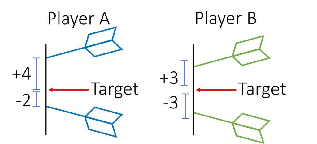
Figure 1. A lateral view of darts thrown by Player A and B on a dartboard.
In this hypothetical scenario, both players missed the target by 3 inches on average. However, neither player appears to play similarly. In this case, the variance may offer a different perspective on analyzing the game results and untying this situation.
The variance is an inflated measure of error that equals the average sum of squares. So the first player’s variance is 10 [(42+22)/2=10], while the variance of the second player is 9 [(32+32)/2=9] . Now that the two players appear to play differently, it appears that player B is the winner because he or she had the lowest error using the variance approach.
Because the variance squares the errors, it penalizes larger errors more severely. For example, a three-unit error yields a variance of 9, whereas a four-unit error yields a variance of 16. As a result, the variance can be used to compare mean errors while also accounting for some of the data dispersion. Although both players (A and B) missed the target by 3 inches on average, Player A threw the dart that was farther from the target, resulting in the greatest variance. Nonetheless, player A threw the dart that was closest to the target as well. As a result, simply analyzing the variance may not be sufficient to declare a winner. We can use analysis of variance in this case.
Analysis of variance
The variance (or average sum of squares) was calculated in the previous example based on a target, which is a reference point that helps to indicate how well the two players play. In most cases, however, there is no target or reference point. To address this issue, the ANOVA generates its own target, which is the mean of all observations. As an example, imagine that Player A and Player B are throwing darts at an empty wall. The target becomes the average of all throws between the players using the ANOVA method, as shown in Figure 2.
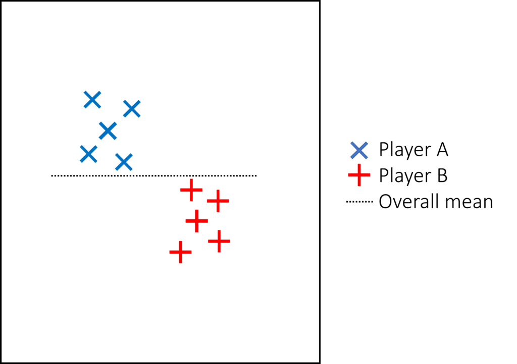
Figure 2. Darts thrown by Player A and B on an empty wall.
As illustrated in Figure 2, an ANOVA assumes that all players attempt to hit the same target. Put another way, the hypothesis is that the groups are similar. This initial hypothesis is known as the Null hypothesis. The analysis then determines, based on the data, whether the two groups are distinct, thus rejecting or not the Null hypothesis. Figure 2 clearly shows that both players were aiming at different targets. However, depending on how dispersed the data is, this distinction may not be discernible. Consider the two scenarios depicted in Figure 3.
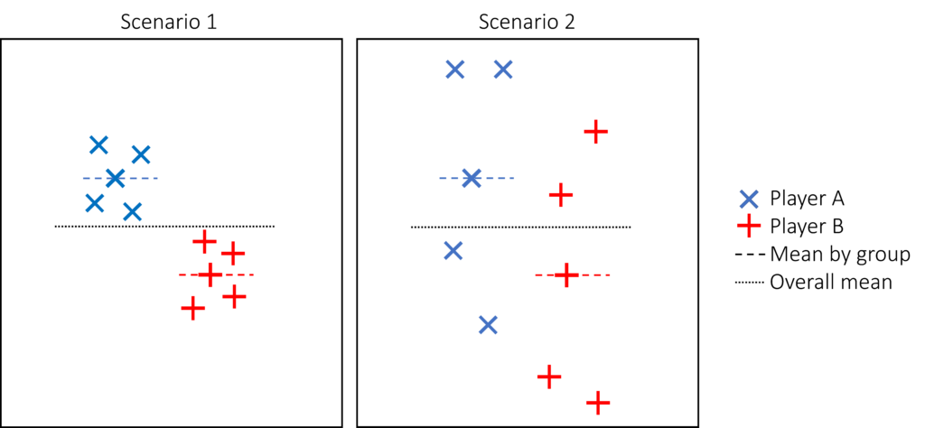
Figure 3. Two different scenarios of darts thrown by Player A and B on an empty wall.
In Scenario 1, it is evident that each player was aiming at different targets, whereas in Scenario 2, this is less apparent, despite the fact that both players missed the target with the same average error. In Scenario 2, it is possible that both players were aiming for the same target, but they are simply poor players. Consequently, in Scenario 2, we cannot be certain. As depicted in Figure 3, dispersion plays a role in analyzing differences between groups. The ANOVA was designed to compare the variance between groups and the variance within groups to account for dispersion. As stated previously, the variance corresponds to the mean sum of squares (SS). Thus, the ANOVA is essentially a test that compares the between-group and within-group SS (Figure 4). Generally speaking, if the ratio of the between-group SS to the within-group SS is greater than 2, differences between groups can be assumed. In the ANOVA test, the ratio of the between-group SS to the within-group SS is referred to as the F-statistic. The larger the F-statistic, the smaller the p-value it produces.
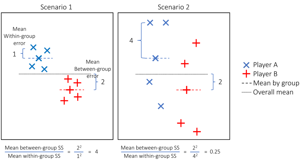
Figure 4. Two different scenarios of darts thrown by Player A and B on an empty wall. The variance or sum of squares between and withing groups are shown and the calculation of the F-statistic.
Despite the fact that there are no differences between the groups in Scenario 2 (F-statistic = 0.25, P>0.05), we cannot accept the Null hypothesis that both groups are similar because we are uncertain. If, in Scenario 2, both groups differ, adding more observations should reduce within-group error because more observations should be close to the true mean of each group. As a result, the F-statistic may rise, revealing group differences. Thus, the differences were not detected because they did not exist, but because there were insufficient observations.
Statistical tests are not intended to validate a Null hypothesis. In essence, a Null hypothesis is an assumption, one that may be incorrect. As a result, the absence of sufficient evidence to refute the assumption does not transform it into a fact. Unfortunately, as discussed in previous posts, there are numerous studies in the animal sciences literature that accept Null hypotheses due to a lack of evidence against them.
The previous ANOVA test calculations were incomplete because the degrees of freedom, which are an important component of the calculations, were not included. Degrees of freedom were discussed in a previous post and will not be revisited here, but they can be summarized as a calculation that accounts for the fact that the sample is only a sample and penalizes it accordingly. Smaller samples are penalized more severely as a result. Degrees of freedom are an important calculation that takes into account the possibility of inaccuracies due to a small sample size in order to make the results more generalizable.
Domain knowledge
Returning to the example shown in Figure 1, which is reproduced below. There should be no differences between groups, according to the ANOVA; the differences between and within SS are insufficient. However, if we consider a standard dartboard, player A scored 43 points and player B scored 23, making player A the clear winner (Figure 5). Similarly, in research, even if two groups are similar and ANOVAs show no differences, the fact that both groups are similar cannot be accepted. Perhaps our initial assumption was incorrect, and we are missing a critical piece of the puzzle (the board).
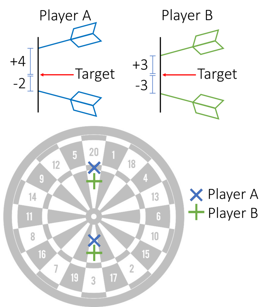
Figure 5. A lateral and frontal view of darts thrown by Player A and B on a dartboard.
As discussed in a previous post, two groups of animals performed similarly when both received diets in excess and deficiencies in the same degree relative to the requirement (Figure 6). The authors concluded that both groups performed similarly because the low protein group was supplemented with amino acids; the lack of evidence contradicting their assumptions confirmed them. In this case, the authors were missing the board, or domain knowledge in the field. ANOVA cannot solve a dose-response problem because both the dose and the response are numerical. The ANOVA test is only adequate when comparing categorical groups, like players. In short, please do not accept Null Hypotheses, even if they make sense to you because the original hypothesis may be incorrect.
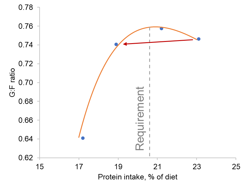
Figure 6. Similar performance can be achieved by two diets that have an equal proportion of excess or deficiency of crude protein relative to the requirement; based on data from [1]. Protein requirement (reported as nitrogen requirement) according to the National Research Council [2].
Thanks for reading, and I hope you found this post helpful! Please, please, please leave a comment to let me know if the post was clear enough.
Christian Ramirez-Camba
1. Yue, L. and S. Qiao, Effects of low-protein diets supplemented with crystalline amino acids on performance and intestinal development in piglets over the first 2 weeks after weaning. Livestock Science, 2008. 115(2-3): p. 144-152.
2. NRC, Nutrient Requirements of Swine: Eleventh Revised Edition. 2012, Washington, DC: The National Academies Press. 420.